
If you’ve been using VLOOKUP in Excel for years, it’s time to meet its smarter, more powerful successor: XLOOKUP. Introduced in Excel 2019 and available in Microsoft 365, XLOOKUP fixes nearly every frustration that VLOOKUP users have ever complained about. Here’s a complete breakdown of how they compare — and why you should switch today.
The Quick Summary
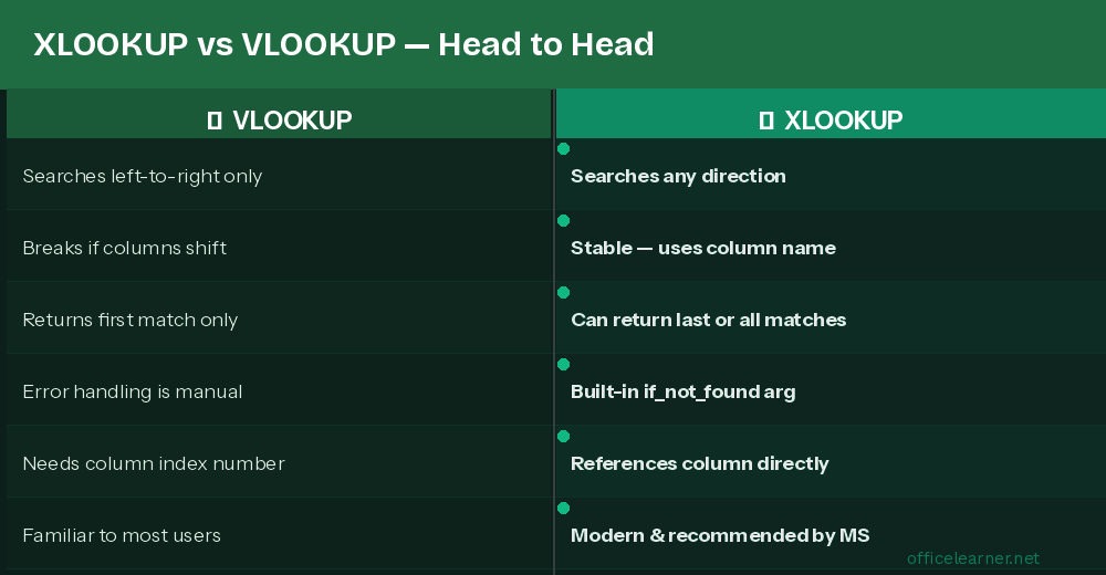
XLOOKUP can search left or right, returns exact matches by default, handles missing values gracefully, and supports arrays natively. VLOOKUP is limited to searching the leftmost column and returning values to its right. For new Excel users, start with XLOOKUP. For existing VLOOKUP users, this guide will make the switch easy.
What Is VLOOKUP?
VLOOKUP (Vertical Lookup) has been an Excel staple since the 1980s. The syntax is:
=VLOOKUP(lookup_value, table_array, col_index_num, [range_lookup])It searches the first column of a table and returns a value from a column to the right, specified by its number. You must count columns manually, and if your data structure changes, your formula breaks.
What Is XLOOKUP?
XLOOKUP is Microsoft’s modern replacement. The syntax is:
=XLOOKUP(lookup_value, lookup_array, return_array, [if_not_found], [match_mode], [search_mode])Instead of specifying a whole table and a column number, you specify exactly which column to search and exactly which column to return. This makes formulas far more readable and flexible.
Key Difference #1: Search Direction
VLOOKUP: Can only search the leftmost column of the table array. If you need to look up a value in column C and return a value from column A (to the left), VLOOKUP simply cannot do it — you’d need INDEX/MATCH instead.
XLOOKUP: Can search any column and return any column, regardless of direction. Searching right-to-left is just as easy as left-to-right. This alone eliminates entire categories of complex workarounds.
Example: Find the Employee Name (column A) by searching their ID (column D):
=XLOOKUP(G2, D:D, A:A)VLOOKUP cannot do this without restructuring your data.
Key Difference #2: Exact Match Default
VLOOKUP: The last argument (range_lookup) defaults to TRUE, meaning approximate match. Forgetting to type FALSE causes wrong results that look correct — one of Excel’s most common and dangerous errors.
=VLOOKUP(A2, B:D, 2, FALSE) ← You must always add FALSEXLOOKUP: Defaults to exact match (match_mode = 0). No extra argument needed for the most common use case. Far fewer accidental errors.
=XLOOKUP(A2, B:B, C:C) ← Exact match by default, clean and simpleKey Difference #3: Handling Missing Values
VLOOKUP: Returns #N/A when no match is found. To handle this, you must wrap it in IFERROR:
=IFERROR(VLOOKUP(A2, B:D, 2, FALSE), "Not Found")XLOOKUP: Has a built-in [if_not_found] argument (the 4th parameter) that handles missing values natively:
=XLOOKUP(A2, B:B, C:C, "Not Found")Cleaner, shorter, and less prone to wrapping errors.
Key Difference #4: Column Referencing
VLOOKUP: Requires a column index number (e.g., 3 for the third column). If you insert or delete columns, the number is wrong and results change silently.
XLOOKUP: References columns directly by name or range (e.g., C:C). Inserting columns doesn’t break your formula because you’re referencing the actual column, not counting to it.
Key Difference #5: Multiple Returns
VLOOKUP: Returns a single value only. To return values from multiple columns, you need separate VLOOKUP formulas for each column.
XLOOKUP: Can return an entire row or array in one formula. Specify a multi-column range as the return_array and XLOOKUP spills the results across multiple cells automatically.
=XLOOKUP(A2, B:B, C:E) ← Returns values from columns C, D, and E in one formulaKey Difference #6: Search Modes
XLOOKUP’s 6th argument lets you control the search direction:
- 1 (default): First-to-last search
- -1: Last-to-first search (great for finding the most recent entry)
- 2: Binary search ascending (faster for large sorted datasets)
- -2: Binary search descending
VLOOKUP has no equivalent flexibility.

When Should You Still Use VLOOKUP?
Honestly, there are very few reasons to use VLOOKUP in 2025. The only real case is compatibility: if you need your workbook to work in Excel 2016 or earlier, XLOOKUP won’t be available. For everything else, XLOOKUP is strictly better.
Quick Migration Guide
Converting your existing VLOOKUP formulas to XLOOKUP is straightforward:
Old: =VLOOKUP(A2, C:F, 3, FALSE)
New: =XLOOKUP(A2, C:C, E:E, "Not Found")
Replace the table_array and col_index_num with the specific lookup_array and return_array columns. Add your “not found” text as the 4th argument and you’re done.
Final Verdict
XLOOKUP is superior to VLOOKUP in every meaningful way. It searches in any direction, defaults to exact match, handles errors natively, doesn’t break when columns are inserted, and can return multiple columns at once. If you’re on Microsoft 365 or Excel 2019+, there’s no reason to keep writing VLOOKUP formulas. Make the switch today — your future self will thank you.


