What is the IF function in Google Sheets?
When you use the IF function, you build a decision tree in which a particular action occurs if a given condition is met, and a different action occurs if the condition is not met.
For this reason, the function’s condition must take the form of an alternative question that can only have the responses “yes” or “no.”
This is what a decision tree may look like:
As a result, the IF function enables you to pose a query and provide one of two potential responses. Three arguments for the function are known as this query and the alternate courses of action.
IF function syntax in Google Sheets
The syntax for the IF function and its arguments are as follows:
=IF(logical_expression, value_if_true, value_if_false)
- logical_expression – (required) a value or logical expression that is tested to see if it is TRUE or FALSE.
- value_if_true – (required) the operation that is carried out if the test is TRUE.
- value_if_false – (optional) the operation that is carried out if the test is FALSE.
Let’s explore the arguments of our IF function in more detail.
The first argument represents a logical question. Google Sheets answers this question with either “yes” or “no”, i.e. “true” or “false”.
How to formulate the question properly, you may wonder? To do that, you can write a logical expression using such helpful symbols (or comparison operators) as “=”, “>”, “<“, “>=”, “<=”, “<>”. Let us try and ask such a question together.
Usage of the IF function
Assume for the moment that you are employed by a business that sells chocolate to several customers in various consumer regions.
This is what your sales data may look like in Google Sheets: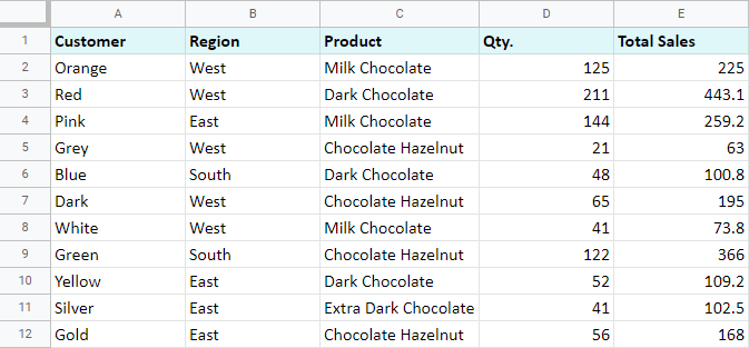
Consider the necessity to distinguish between domestic and international sales. To do that, add a new field that describes the country in which each sale was made for each sale. You need this description field to be generated automatically for each entry because there is a lot of data.
And at this point, the IF function is used. Let’s add a column called “Country” to the data table. The “West” region reflects domestic sales, while the remaining areas indicate international sales (Rest of the World).
How to write out the function properly?
Place the cursor in F2 to make the cell active and type in the equality sign (=). Google Sheets will immediately understand that you are going to enter a formula. That’s why right after you type the letter “i” it will prompt you to choose a function that begins with that same letter. And you should choose “IF”.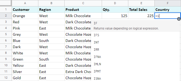
After that, all your actions will be accompanied by prompts as well.
For the first argument of the IF function, enter B2=”West”. As with the other Google Sheets functions, you don’t need to enter the address of the cell manually – a mouse click is enough. Then enter comma (,) and specify the second argument.
The second argument is a value that F2 will return if the condition is met. In this case, it will be the text “Our Country”.
And again, after the comma, write the value of the 3rd argument. F2 will return this value if the condition is not met: “Rest of the World”. Do not forget to finish your formula entry by closing parenthesis “)” and pressing “Enter”.
Your entire formula should look like this:
=IF(B2="West","Our Country","Rest of the World")
If everything is correct, F2 will return the text “Our Country”: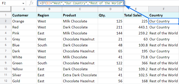
Now, all you have to do is to copy this function down column F.
Tip. There’s one way to process the entire column with one formula. The ARRAYFORMULA function will help you do that. Using it in the first cell of the column, you can test all cells below against the same condition, and return the corresponding result to each row at the same time:
=ARRAYFORMULA(IF(B2:B69="West","Our Country","Rest of the World"))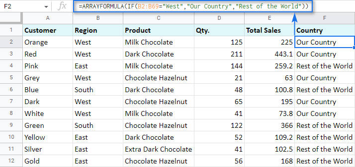
Let’s examine the other ways of working with the IF function.
IF function and text values
The usage of the IF function with a text has already been illustrated in the example above.
Note. If the text is being used as the argument, then it must be enclosed in double-quotes.
IF function and numerical values
You can use numbers for the arguments just as you did with the text.
However, what is very important here is that the IF function makes it possible to not only fill cells with certain numbers based on the conditions met but also calculate.
For example, let’s say you offer your clients various discounts based on the total value of the purchase. If the total is more than 200, then the client gets a 10% discount.
For that, you need to use column G and name it “Discount”. Then enter the IF function in G2, and the second argument will be represented by the formula that calculates the discount:
=IF(E2>200,E2*0.1,0)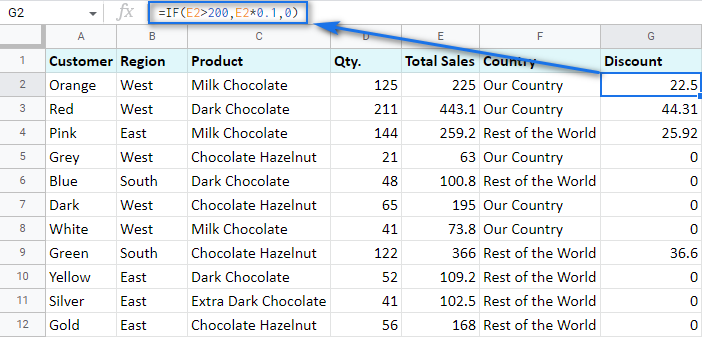
IF blanks/non-blanks
There are cases when your result depends on whether the cell is empty or not. There are two ways to check that:
- Use the ISBLANK function.For example, the following formula checks if cells in column E are empty. If so, no discount should be applied, otherwise, it’s 5% off:
=IF(ISBLANK(E2)=TRUE,0,0.05)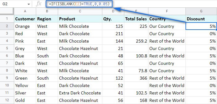 Note. If there’s a zero-length string in a cell (returned by some formula), the ISBLANK function will result in FALSE.Here is another formula to check if E2 is empty:
=IF(ISBLANK(E2)2<>FALSE,0,0.05)You can turn the formula the other way around and see if cells are not blank instead:=IF(ISBLANK(E2)=FALSE,0.05,0=IF(ISBLANK(E2)<>TRUE,0.05,0) - Use standard comparison operators with a pair of double-quotes:Note. This method considers zero-length strings (indicated by double-quotes) as empty cells.
=IF(E2="",0,0.05)– check if E2 is blank=IF(E2<>"",0,0.05)– check if E2 is not empty.Tip. In a similar manner, use double-quotes as an argument to return an empty cell by the formula:=IF(E2>200,E2*0,"")
IF in combination with other functions
As you have already learned, the text, numbers, and formulas can act as the arguments of the IF function. However, other functions can play that role as well. Let’s see how it works.
Google Sheets IF OR
Remember the first way you figured out the country where you sold chocolate? You checked if B2 contained “West”.
However, you can build the logic the other way around: list all the possible regions that belong to the “Rest of the World” and check if at least one of them appears in the cell. The OR function in the first argument will help you do that:
=OR(logical_expression1, [logical_expression2, …])
- logical_expression1 – (required) the first logical value to check for.
- logical_expression2 – (optional) the next logical value to check for.
- and so on.
As you can see, you just enter as many logical expressions as you need to check and the function searches if one of them is true.
To apply this knowledge to the table with sales, mention all the regions that belong to the sales abroad, and the other sales will automatically become local:
=IF(OR(B2="East",B2="South"),"Rest of the World","Our Country")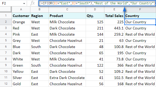
Google Sheets IF AND
The AND function is just as simple. The only difference is that it checks if all listed logical expressions are true:
=AND(logical_expression1, [logical_expression2, …])
E.g. you need to narrow the search to your town and you know that it is currently buying only hazelnuts. So there are two conditions to consider: region – “West” and product – “Chocolate Hazelnut”:
=IF(AND(B2="West",C2="Chocolate Hazelnut"),"Our Country","Rest of the World")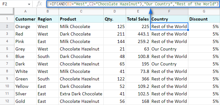
Nested IF formula vs. IFS function for Google Sheets
You can also use the IF function itself as an argument for the bigger IF function.
Let’s assume that you have set stricter discount conditions for your clients. If the total purchase is more than 200 units, they get a 10% discount; if the total purchase is between 100 and 199, the discount is 5%. If the total purchase is lower than 100, there is no discount whatsoever.
The following formula shows how the function will look in the cell G2:
=IF(E2>200,E2*0.1,IF(E2>100,E2*0.05,0))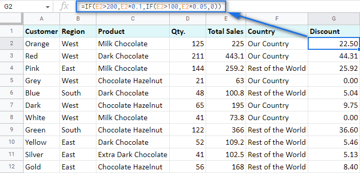
Note that it is another IF function that is used as the second argument. In such cases, the decision tree is as follows:
Let’s make it even more fun and complicate the task. Imagine that you’re offering the discounted price to the one region only – “East”.
To do that correctly, add the logical expression “AND” to our function. The formula then will look the following way:
=IF(AND(B2="East",E2>200),E2*0.1,IF(AND(B2="East",E2>100),E2*0.05,0))
As you can see, the number of discounts has reduced greatly while their amount remains intact.
There’s also an easier way to write the above thanks to the IFS function:
=IFS(condition1, value1, [condition2, value2, …])
- condition1 – (required) is the logical expression you want to test.
- value1 – (required) is the value to return if the condition1 is true.
- and then you just list conditions with their values to return if they are true.
Here’s how the above formula will look with IFS:
=IFS(AND(B2="East",E2>200),E2*0.1,AND(B2="East",E2>100),E2*0.05)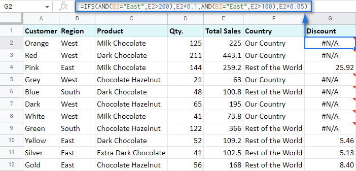
Tip. If there’s no true condition, the formula will return the #N/A error. To avoid that, wrap your formula with IFERROR:
=IFERROR(IFS(AND(B2="East",E2>200),E2*0.1,AND(B2="East",E2>100),E2*0.05),0)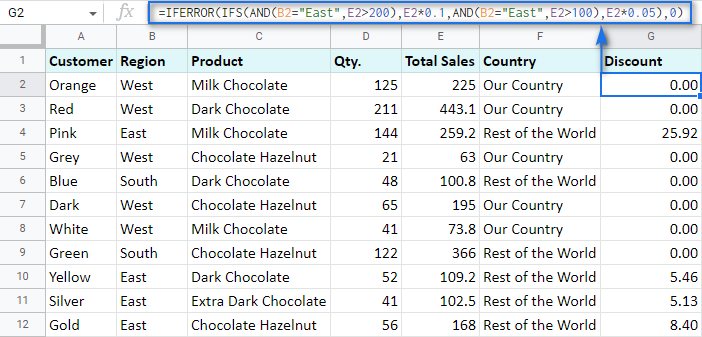
SWITCH as an alternative to multiple IFs
There’s one more function you may want to consider instead of the nested IF: Google Sheets SWITCH.
It checks if your expression corresponds to a list of cases, one by one. When it does, the function returns a corresponding value.
=SWITCH(expression, case1, value1, [case2, value2, …], [default])
- expression is any cell reference, or a range of cells, or even an actual math expression, or even a text that you’d like to equal to your cases (or test against the criteria). Required.
- case1 is your first criteria to check the expression against. Required.
- value1 is a record to return if the case1 criterion is the same as your expression. Required.
- case2, value2 repeat as many times as criteria you have to check and values to return. Optional.
- default is also completely optional. Use it to see a specific record if none of the cases is met. I’d recommend using it every time to avoid errors when your expression doesn’t meet matches among all the cases.
Here are a couple of examples.
To test your cells against a text, use ranges as an expression:
=ARRAYFORMULA(SWITCH(B2:B69,"West","Our Country","Rest of the World"))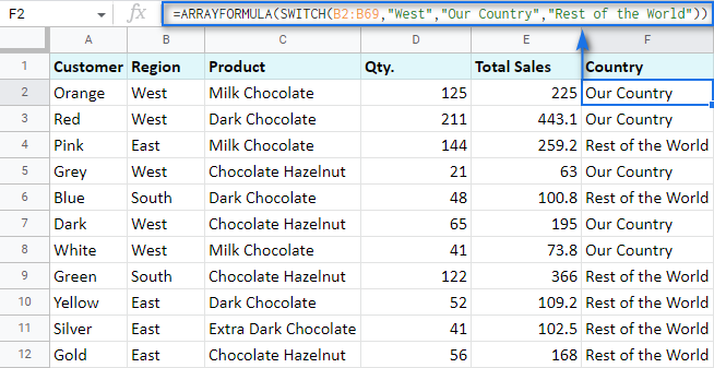
In this formula, SWITCH checks what record is in every cell in column B. If it’s West, the formula says Our Country, otherwise, Rest of the World. ArrayFormula makes it possible to process the entire column at once.
To work with calculations, it’s better to use a boolean expression:
=SWITCH(TRUE,$E2>200,$E2*0.1,AND($E2<200,$E2>100),$E2*0.05,0)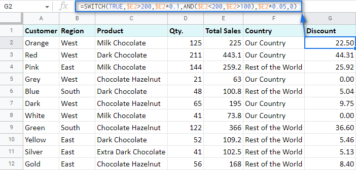
Here SWITCH checks if the result of the equation is TRUE or FALSE. When it’s TRUE (like if E2 is really greater than 200), I get a corresponding result. If none of the cases in the list is TRUE (meaning they are FALSE), the formula simply returns 0.
Note. SWITCH doesn’t know how to calculate the entire range at once, so no ARRAYFORMULA in this case.
IF statements based on a count
One of the questions we get asked a lot is how to create the IF formula that will return whatever you need if the column contains or doesn’t contain a certain record.
For example, check if a customer’s name appears more than once in a list (column A) and put the corresponding word (yes/no) into a cell.
A solution is simpler than you may think. You need to introduce the COUNTIF function to your IF:
=IF(COUNTIF($A$2:$A$20,$A2)>1,"yes","no")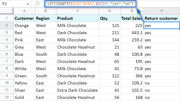
Make Google Sheets build IF formulas for you – IF Formula Builder add-on
If you’re tired of keeping track of all those extra characters and proper syntax in formulas, there’s another solution available.
IF Formula Builder add-on for Google Sheets offers a visual way of creating IF statements. The tool will handle syntax, extra functions and all required characters for you.
All you need to do is:
- fill blanks with your records one by one. No special treatment for dates, time, etc. Enter them as you always do and the add-on will recognize the data type.
- select required comparison operators from the suggested drop-down lists.
- if needed, add multiple logical expressions in a click: IF OR, IF AND, ELSE IF, THEN IF.
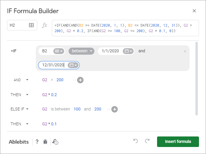
As you can see, each logical expression takes its own line. The same goes for true/false outcomes. This reduces the number of possible confusion over the formula drastically.
As you fill everything out, the formula for use will grow in the preview area at the top of the window. To its left, you can select a cell in your sheet where you’d like to have the formula.
When you’re ready, paste the formula into the cell of interest by clicking the Insert formula button at the bottom.
Please visit the online tutorial for IF Formula Builder to see all options described in detail.
I hope that there’s no room for any doubt now that the IF function, though a very simple one at first glance, opens the door to many options for data processing in Google Sheets. But if you still have questions, feel free to ask them in the comments section down below – we’ll be happy to help!


